Introduction

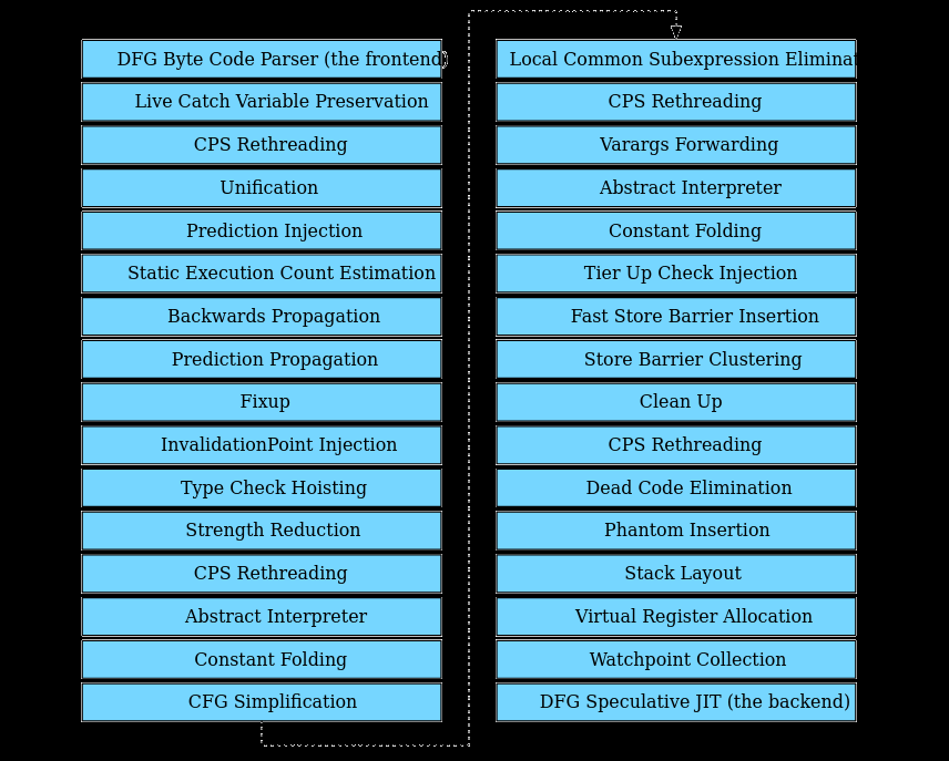
This blog post continues from where we left off in Part III and will cover each DFG graph optimisation. The graph generated at the end of the bytecode parsing phase is passed through the DFG pipeline which optimises the graph before lowering it to machine code. DFG Optimisation phases add, remove and update nodes in the various blocks that make up the graph. The optimisation phases will also re-order nodes (via Hoisting or Sinking) within the same basic block. However, the DFG optimisations do not move nodes between basic blocks. The the screenshot¹ below shows the various optimisation phases that form part of the DFG pipeline:

dfg-optimisation

The goal of DFG optimisation is to enable Fast Compilation by removing as many type checks as possible, quickly. The DFG performs majority of its optimisations via static analysis of the generated graph. The WebKit blog¹ describes three key static analyses in the DFG that have a significant impact on optimisation choices:

We use prediction propagation to fill in predicted types for all values based on value profiling of some values. This helps us figure out where to speculate on type.

We use the abstract interpreter (or just AI for short in JavaScriptCore jargon) to find redundant OSR speculations. This helps us emit fewer OSR checks. Both the DFG and FTL include multiple optimization passes in their pipelines that can find and remove redundant checks but the abstract interpreter is the most powerful one. The abstract interpreter is the DFG tier’s primary optimization and it is reused with small enhancements in the FTL.

We use clobberize to get aliasing information about DFG operations. Given a DFG instruction, clobberize can describe the aliasing properties. In almost all cases that description is O(1) in time and space. That description implicitly describes a rich dependency graph.

Graph Optimisations

The DFG pipeline itself has 30 optimisation passes of which 25 are unique optimisation phases. The optimisation phases indicated previously are located in DFGPlan.cpp.

    RUN_PHASE(performLiveCatchVariablePreservationPhase);

    RUN_PHASE(performCPSRethreading);
    RUN_PHASE(performUnification);
    RUN_PHASE(performPredictionInjection);
    
    RUN_PHASE(performStaticExecutionCountEstimation);

    //... truncated for brevity

With a high level understanding of the three static analysis performed, let’s now dive into the details of each optimisation phase. To being, there are a couple of command line line flags that one can add to our debugging environment that will aid our evaluation:

verboseCompilation: This flag will enable printing of logging information at before and after each optimisation phase of the DFG. This will also help identify which optimisation phase the DFG is currently in and if the phase modified the DFG IR. This will also print the final optimised graph at the end of the optimisation phases.
dumpGraphAtEachPhase: As the name suggests, setting this flag will enable printing of the graph at the start of each optimisation phase.

Our launch.json should resemble something similar to the one below:

{
    //... trunvated for brevity
           "program": "/home/amar/workspace/WebKit/WebKitBuild/Debug/bin/jsc",
            "args": [
                "--useConcurrentJIT=false",
                "--useFTLJIT=false",
                "--verboseOSR=true",

                "--thresholdForJITSoon=10", 
                "--thresholdForJITAfterWarmUp=10", 
                "--thresholdForOptimizeAfterWarmUp=100", 
                "--thresholdForOptimizeAfterLongWarmUp=100", 
                "--thresholdForOptimizeSoon=100", 

                "--reportDFGCompileTimes=true",     
                "--dumpBytecodeAtDFGTime=true",
                "--dumpSourceAtDFGTime=true",
                "--verboseDFGBytecodeParsing=false", 
                "--dumpGraphAfterParsing=false",
                
                "--dumpGraphAtEachPhase=true",
                "--verboseCompilation=true",
                
                "/home/amar/workspace/WebKit/WebKitBuild/Debug/bin/test.js"
            ],
    //... truncated for brevity
}

Live Catch Variable Preservation

The first optimisation phase in the pipeline is LiveCatchVariablePreservationPhase. The header files for each phase include developer comments on the function of the optimistaion phase. The LiveCatchVariablePreservationPhase is described by the developer comments as follows:

This phase ensures that we maintain liveness for locals that are live in the “catch” block. Because a “catch” block will not be in the control flow graph, we need to ensure anything live inside the “catch” block in bytecode will maintain liveness inside the “try” block for an OSR exit from the “try” block into the “catch” block in the case of an exception being thrown.

The mechanism currently used to demonstrate liveness to OSR exit is ensuring all variables live in a “catch” are flushed to the stack inside the “try” block.

This phase iterates over each basic block in the graph and attempts to determine which operands from the catch block would need to be preserved in the graph so that at the time of OSR Exit, the catch block can be correctly reconstructed in the Baseline JIT. Live values in the DFG relevant to the catch block are preserved by inserting Flush nodes at the end of the basic block which will push these values to the stack. Flush nodes ensure that the DFG optimisation will preserve the value of an operand at OSR Exit.

The function performLiveCatchVariablePreservationPhase is implemented as the run function. A snippet of which is shown below:

bool run()
{
    DFG_ASSERT(m_graph, nullptr, m_graph.m_form == LoadStore);

    if (!m_graph.m_hasExceptionHandlers)
        return false;

    InsertionSet insertionSet(m_graph);
    if (m_graph.m_hasExceptionHandlers) {
        for (BasicBlock* block : m_graph.blocksInNaturalOrder()) {
            handleBlockForTryCatch(block, insertionSet);
            insertionSet.execute(block);
        }
    }

    return true;
}

The object insertionSet is an ordered collection of new nodes that are generated when the graph is put through an optimisation phase. At the end of the phase, the insertionSet is executed which adds these new nodes to the various basic blocks in the graph.

CPS Rethreading

The next stage in the optimistaion pipeline is CPSRethreading. Before this stage the graph generated is in the LoadStore form and this phase converts the graph to a ThreadedCPS form. The properties of a ThreadedCPS graph are described as follows:

ThreadedCPS form means that basic blocks list up-front which locals they expect to be live at the head, and which locals they make available at the tail. ThreadedCPS form also implies that:

GetLocals and SetLocals are not redundant within a basic block.

All GetLocals and Flushes are linked directly to the last access point of the variable, which must not be another GetLocal.

Phantom(Phi) is not legal, but PhantomLocal is.

ThreadedCPS form is suitable for data flow analysis (CFA, prediction propagation), register allocation, and code generation.

Before we dive into the phase implementation, it’s worth reviewing the functionality of some of the most common nodes in a graph:

MovHint(@a, rK): This operation indicates that node @a contains the value that would have now been placed into virtual register rK. Does not actually cause @a to be stored into rK. MovHints are always dead.
SetLocal(@a, rK): This is a store operation that causes the result of @a is stored to the virtual register rK, if the SetLocal is live.
GetLocal(@a, rK): This is a load operation that causes the result of @a to be loaded from the virtual register rK.

The developer comments describe the phase as follows:

CPS Rethreading:

Takes a graph in which there are arbitrary GetLocals/SetLocals with no connections between them. Removes redundant ones in the case of uncaptured variables. Connects all of them with Phi functions to represent live ranges.

The phase implementation consists of a series of function calls which transform the graph. The functions that perform key transformations are briefly described below:

bool run()
{
    RELEASE_ASSERT(m_graph.m_refCountState == EverythingIsLive);
        
    if (m_graph.m_form == ThreadedCPS)
        return false;
        
    clearIsLoadedFrom();
    freeUnnecessaryNodes();
    m_graph.clearReplacements();
    canonicalizeLocalsInBlocks();
    specialCaseArguments();
    propagatePhis<OperandKind::Local>();
    propagatePhis<OperandKind::Argument>();
    propagatePhis<OperandKind::Tmp>();
    computeIsFlushed();
        
    m_graph.m_form = ThreadedCPS;
    return true;
}

freeUnnecessaryNodes: Adds an empty child node to GetLocal, Flush and PhantomLocal nodes in the graph. When iterating through the nodes in the graph, if it encounters a Phantom node it removes the node if the node has no children. If the node has a child which is either a Phi, SetArgumentDefinitely or a SetLocal, it converts the node to a PhantomLocal. At the end of parsing each block it purges any Phi nodes that exist from previous optimisation passes.

canonicalizeLocalsInBlocks: This function defines the rules for threaded CPS. Basic Block evaluation begins from the last basic block in the graph to and terminates at the root block. Nodes within each block however are parsed in natural order. This phase is also responsible for updating the varaiblesAtHead list as well as generating (also regenerating since this phase is called several times in the DFG pipeline) Phi nodes and adding them to the graph. The Phi nodes generated can be viewed from the graph dump printed to stdout, an example of this is shown below:

: Block #5 (bc#463 --> isFinite#DJEgRe:<0x7fffaefc7b60> bc#21):
:   Execution count: 1.000000
:   Predecessors: #4
:   Successors: #6
:   Phi Nodes: D@559<loc39,1>->(), D@558<loc40,1>->(), D@557<loc5,1>->(), D@556<this,1>->()
:   States: StructuresAreWatched, CurrentlyCFAUnreachable
:   Vars Before: <empty>
//... truncated for brevity
:   Var Links: arg0:D@592 loc5:D@593 loc39:D@464 loc40:D@465

In the snippet above D@559 is a Phi node that’s been added to the graph. The value loc39 represents the operand to Phi node. The value 1 that follows loc39 is the reference count for the Phi.

propogatePhis: This group of functions propagates Phi nodes through the basic blocks. This propagation process updates the Phi nodes with child nodes from a predecessor block who’s value would flow into the Phi node.

//... truncated for brevity
4   :    D@427:< 1:->      SetLocal(Check:Untyped:D@410, loc40(FF~/FlushedJSValue), W:Stack(loc40), bc#0, ExitValid)  predicting None
4   :    D@428:< 1:->      SetLocal(Check:Untyped:D@423, loc39(GF~/FlushedJSValue), W:Stack(loc39), bc#0, ExitValid)  predicting None
//... truncated for brevity

5   : Block #5 (bc#463 --> isFinite#DJEgRe:<0x7fffaefc7b60> bc#21):
5   :   Execution count: 1.000000
5   :   Predecessors: #4
5   :   Successors: #6
5   :   Phi Nodes: D@559<loc39,1>->(D@428), D@558<loc40,1>->(D@427), D@557<loc5,1>->(D@554), D@556<this,1>->(D@553), D@655<loc23,1>->(D@651), D@650<loc24,1>->(D@646), D@165<loc26,1>->(D@409), D@680<loc34,1>->(D@403), D@684<loc30,1>->(D@397), D@688<loc4,1>->(D@555), D@696<arg1,1>->(D@700), D@703<arg2,1>->(D@707)
5   :   States: StructuresAreWatched, CurrentlyCFAUnreachable
5   :   Vars Before: <empty>
     //... truncated for brevity
5   :   Var Links: arg2:D@703 arg1:D@696 arg0:D@592 loc4:D@688 loc5:D@593 loc23:D@655 loc24:D@650 loc26:D@165 loc30:D@684 loc34:D@680 loc39:D@464 loc40:D@465

In the snippet above the Phi node D@559 has an edge to the child node pointing to the SetLocal node D@428 which is in the predecessor block #4. The children of a Phi node can only be SetLocal, SetArgumentDefinitely, SetArgumentMaybe or another Phi node.

Unification

Examines all Phi functions and ensures that the variable access datas are unified. This creates our “live-range split” view of variables.

This phase iterates over all Phi nodes and attempts to unify the VariableAccessData for the Phi nodes and the children of the node.

for (unsigned phiIndex = block->phis.size(); phiIndex--;) {
    Node* phi = block->phis[phiIndex];
    for (unsigned childIdx = 0; childIdx < AdjacencyList::Size; ++childIdx) {
        if (!phi->children.child(childIdx))
            break;
        phi->variableAccessData()->unify(phi->children.child(childIdx)->variableAccessData());
    }
}

If the child node has a different VariableAccessData to the parent then then the child is made the parent of the Phi node. The snippet from WebKit/WebKitBuild/Debug/DerivedSources/ForwardingHeaders/wtf/UnionFind.h:

void unify(T* other)
{
    T* a = static_cast<T*>(this)->find();
    T* b = other->find();
        
    ASSERT(!a->m_parent);
    ASSERT(!b->m_parent);
        
    if (a == b)
        return;
        
    a->m_parent = b;
}

VariableAccessData contains operand information and are stored in a vector defined in dfg/DFGGraph.h.

SegmentedVector<VariableAccessData, 16> m_variableAccessData;

The DFG nodes, SetArgumentDefinitely, SetArgumentMaybe, GetLocal and SetLocal store VariableAccessData as an opInfo parameter. This can be retrieved with a call to node->tryGetVariableAccessData(). See Graph::dump for the VariableAccessData dumping section.

Prediction Injection

Takes miscellaneous data about variable type predictions and injects them. This includes argument predictions and OSR entry predictions.

As the developer comments suggest, this phase takes the the profiling data collected from the profiling tier and then injects them into the IR. This affects GetLocal, SetLocal and Flush nodes. As an example, let’s consider nodes generated for an arithmetic add instruction whose operands have been profiled as integer values:

D@28:<!0:-> GetLocal(JS|MustGen|PureInt, arg1(B~/FlushedJSValue), R:Stack(arg1), bc#7, ExitValid)  predicting None
D@29:<!0:-> GetLocal(JS|MustGen|PureInt, arg2(C~/FlushedJSValue), R:Stack(arg2), bc#7, ExitValid)  predicting None
D@30:<!0:-> ValueAdd(Check:Untyped:D@28, Check:Untyped:D@29, JS|MustGen|PureInt, R:World, W:Heap, Exits, ClobbersExit, bc#7, ExitValid)

Prediction Injection phase takes the profile information gathered for each block (e.g. arguments to the block) and injects this to the node. From the snippet above, the nodes D@28 and D@29 above, after prediction injection, would be updated as follows:

D@28:<!0:-> GetLocal(Check:Untyped:D@1, JS|MustGen|PureInt, arg1(B~<BoolInt32>/FlushedJSValue), R:Stack(arg1), bc#7, ExitValid)  predicting BoolInt32
D@29:<!0:-> GetLocal(Check:Untyped:D@2, JS|MustGen|PureInt, arg2(C~<Int32>/FlushedJSValue), R:Stack(arg2), bc#7, ExitValid)  predicting NonBoolInt32
D@30:<!0:-> ValueAdd(Check:Untyped:D@28, Check:Untyped:D@29, JS|MustGen|PureInt, R:World, W:Heap, Exits, ClobbersExit, bc#7, ExitValid)

Notice how the graph now contains predicted types for arg1 and arg2 which is BoolInt32 and Int32 respectively. Additionally, it has added prediction information that the nodes D@28 and D@29 will result in generating BoolInt32 and NonBoolInt32 types.

D@28: ... arg1(B~<BoolInt32>/FlushedJSValue) ... predicting BoolInt32

D@29: ... arg2(C~<Int32>/FlushedJSValue) ... predicting NonBoolInt32

Static Execution Count Estimation

Estimate execution counts (branch execution counts, in particular) based on presently available static information. This phase is important because subsequent CFG transformations, such as OSR entrypoint creation, perturb our ability to do accurate static estimations. Hence we lock in the estimates early. Ideally, we would have dynamic information, but we don’t right now, so this is as good as it gets.

This phase adds the static execution counts to each block as well as adds execution weights to each branch and switch node.This phase also calculates dominators for the various blocks in the graph, this is useful for the CFG Simplification phase. See details about this in WebKit/WebKitBuild/Debug/DerivedSources/ForwardingHeaders/wtf/Dominators.h. An example of this is is shown in the graph dump below:

: Block #7 (bc#463 --> isFinite#DJEgRe:<0x7fffaefc7b60> bc#23):
:   Execution count: 1.000000
:   Predecessors: #4
:   Successors: #8 #9
:   Dominated by: #root #0 #2 #3 #4 #7
:   Dominates: #7 #8 #9
:   Dominance Frontier: #6
:   Iterated Dominance Frontier: #6
//... truncated for brevity
:    D@473:<!0:-> MovHint(Check:Untyped:D@472, MustGen, loc54, W:SideState, ClobbersExit, bc#23, ExitValid)
:    D@474:< 1:-> SetLocal(Check:Untyped:D@472, loc54(YF~/FlushedJSValue), W:Stack(loc54), bc#23, exit: bc#463 --> isFinite#DJEgRe:<0x7fffaefc7b60> bc#27, ExitValid)  predicting None
:    D@475:<!0:-> Branch(Check:Untyped:D@472, MustGen, T:#8/w:1.000000, F:#9/w:1.000000, W:SideState, bc#27, ExitValid)

Backwards Propagation

Infer basic information about how nodes are used by doing a block-local backwards flow analysis.

This phase starts by looping over the blocks in the graph from the last to the first and evaluates the NodeFlags on each node. For each node evaluated, it attempts to merge the flags of the node with the NodeBytecodeBackPropMask flags:

void propagate(Node* node)
{
    NodeFlags flags = node->flags() & NodeBytecodeBackPropMask;
        
    switch (node->op()) {
    case GetLocal: {
        VariableAccessData* variableAccessData = node->variableAccessData();
        flags &= ~NodeBytecodeUsesAsInt; // We don't care about cross-block uses-as-int.
        m_changed |= variableAccessData->mergeFlags(flags);
        break;
    }
            
    case SetLocal: {
        VariableAccessData* variableAccessData = node->variableAccessData();
        if (!variableAccessData->isLoadedFrom())
            break;
        flags = variableAccessData->flags();
        RELEASE_ASSERT(!(flags & ~NodeBytecodeBackPropMask));
        flags |= NodeBytecodeUsesAsNumber; // Account for the fact that control flow may cause overflows that our modeling can't handle.
        node->child1()->mergeFlags(flags);
        break;
    }
    //... truncated for brevity
    }
}

Backwards Propagation updates the node flags to provide additional information on how the resultant computation of a node is used.

Prediction Propagation

Propagate predictions gathered at heap load sites by the value profiler, and from slow path executions, to generate a prediction for each node in the graph. This is a crucial phase of compilation, since before running this phase, we have no idea what types any node (or most variables) could possibly have, unless that node is either a heap load, a call, a GetLocal for an argument, or an arithmetic op that had definitely taken slow path. Most nodes (even most arithmetic nodes) do not qualify for any of these categories. But after running this phase, we’ll have full information for the expected type of each node.

Consider the following graph snippet for an arithmetic add operation before the Prediction Propagation phase:

D@28:<!0:-> GetLocal(Check:Untyped:D@1, JS|MustGen|PureInt, arg1(B~<BoolInt32>/FlushedJSValue), R:Stack(arg1), bc#7, ExitValid)  predicting BoolInt32
D@29:<!0:-> GetLocal(Check:Untyped:D@2, JS|MustGen|PureInt, arg2(C~<Int32>/FlushedJSValue), R:Stack(arg2), bc#7, ExitValid)  predicting NonBoolInt32
D@30:<!0:-> ValueAdd(Check:Untyped:D@28, Check:Untyped:D@29, JS|MustGen|PureInt, R:World, W:Heap, Exits, ClobbersExit, bc#7, ExitValid)

The Prediction Propagation phase then traverses the graph to add additional speculative type information on the node itself. The nodes D@28, D@29 and D@30 after the prediction propagation phase are listed below:

D@28:<!0:-> GetLocal(Check:Untyped:D@1, JS|MustGen|PureNum, BoolInt32, arg1(B<BoolInt32>/FlushedInt32), R:Stack(arg1), bc#7, ExitValid)  predicting BoolInt32
D@29:<!0:-> GetLocal(Check:Untyped:D@2, JS|MustGen|PureNum, NonBoolInt32, arg2(C<Int32>/FlushedInt32), R:Stack(arg2), bc#7, ExitValid)  predicting NonBoolInt32
D@30:<!0:-> ArithAdd(Check:Int32:D@28, Check:Int32:D@29, JS|MustGen|PureInt, Int32, Unchecked, Exits, bc#7, ExitValid)

In the listing above, notice the two changes to the node D@30, it now contains speculative type information on what the opcode is likely to return. Which in this case is Int32. It has also updated (technically this is the Fixup phase that updates the node as a consequence of the Prediction Propagation phase) the node to an ArithAdd node type and added an Int32 type check on the edges D@28 and D@29.

ArithAdd(Check:Int32:D@28, Check:Int32:D@29 ...

The nodes D@28 and D@29 have also been updated to include speculative type information for each of them.

Fixup

Fix portions of the graph that are inefficient given the predictions that we have. This should run after prediction propagation but before CSE.

This phase performs a number of optimisations on the graph such as updating the flush formats, type checks, adding nodes (e.g. adding DoubleRep and ArrayifyToStructure) and removing nodes (e.g. decaying Phantoms to Checks). An example of such a node optimisation is the conversion of the ValueAdd node to to a ArithAdd node and the removal of type checks on the node’s children as see in the previous section on Prediction Propagation.

The Fixup rules are defined in the phase implementation. The key functions within the phase that the reader should examine are fixupNode, fixupGetAndSetLocalsInBlock and fixupChecksInBlock.

Invalidation Point Injection

Inserts an invalidation check at the beginning of any CodeOrigin that follows a CodeOrigin that had a call (clobbered World).

As the name of this phase suggests, it adds InvalidationPoint nodes after a node, which has had a call to clobberWorld. InvalidationPoints check if any watchpoints have fired and as a result would trigger an OSR Exit from the optimised code. Consider the following graph dump:

D@287:< 1:-> SetLocal(Check:Untyped:D@284, loc24(QD~<Object>/FlushedJSValue), W:Stack(loc24), bc#283, exit: bc#291, ExitValid)  predicting OtherObj
D@288:<!0:-> PutById(Check:Cell:D@284, Check:Untyped:D@275, MustGen, cachable-id {uid:(__proto__)}, R:World, W:Heap, Exits, ClobbersExit, bc#291, ExitValid)
D@730:<!0:-> InvalidationPoint(MustGen, W:SideState, Exits, bc#297, ExitValid)
D@289:<!0:-> MovHint(Check:Untyped:D@241, MustGen, loc24, W:SideState, ClobbersExit, bc#297, ExitValid)

An InvalidationPoint was added at the beginning of the bytecode instruction boundary at bc#297 since the DFG node PutById triggers a call to clobberWorld when evaluated by the Abstract Interpreter.

Type Check Hoisting

Hoists CheckStructure on variables to assignments to those variables, if either of the following is true:

A) The structure’s transition watchpoint set is valid.

B) The span of code within which the variable is live has no effects that might clobber the structure.

This phase begins by looping over the nodes in the graph to identify any variables with redundant structure and array checks and earmarks their checks for hoisting. It then loops over the SetArgumentDefinitely and SetLocal nodes in the graph and adds CheckStructure nodes on the variables that were earmarked for hoisting. A truncated snippet of the phase implementation is listed below:

bool run()
{
    clearVariableVotes();
    identifyRedundantStructureChecks();
    disableHoistingForVariablesWithInsufficientVotes<StructureTypeCheck>();

    clearVariableVotes();
    identifyRedundantArrayChecks();
    disableHoistingForVariablesWithInsufficientVotes<ArrayTypeCheck>();

    disableHoistingAcrossOSREntries<StructureTypeCheck>();
    disableHoistingAcrossOSREntries<ArrayTypeCheck>();

    bool changed = false;

    // Place CheckStructure's at SetLocal sites.
    InsertionSet insertionSet(m_graph);
    for (BlockIndex blockIndex = 0; blockIndex < m_graph.numBlocks(); ++blockIndex) {
        BasicBlock* block = m_graph.block(blockIndex);
            
        //... truncated for brevity

        for (unsigned indexInBlock = 0; indexInBlock < block->size(); ++indexInBlock) {
            Node* node = block->at(indexInBlock);
                
            //... truncated for brevity

            switch (node->op()) {
            case SetArgumentDefinitely: {
                //... truncated for brevity (GetLocal and CheckStructure/CheckArray nodes added)
            }    
            case SetLocal: {
                //... truncated for brevity (CheckStructure/CheckArray nodes added)
            }    
            default:
                break;
            }
        }
        insertionSet.execute(block);
    }
        
    return changed;
}

Strength Reduction

Performs simplifications that don’t depend on CFA or CSE but that should be fixpointed with CFA and CSE.

The developer comments in DFGStrengthReductionPhase.h aren’t very descriptive on how this phase optimises the graph. However, on digging into the ChangeLog from 2014, we have the following comments that shed more light on what this phase was designed to accomplish:

This was meant to be easy. The problem is that there was no good place for putting the folding of typedArray.length to a constant. You can’t quite do it in the bytecode parser because at that point you don’t yet know if typedArray is really a typed array. You can’t do it as part of constant folding because the folder assumes that it can opportunistically forward-flow a constant value without changing the IR; this doesn’t work since we need to first change the IR to register a desired watchpoint and only after that can we introduce that constant. We could have done it in Fixup but that would have been awkward since Fixup’s code for turning a GetById of “length” into GetArrayLength is already somewhat complex. We could have done it in CSE but CSE is already fairly gnarly and will probably get rewritten.

So I introduced a new phase, called StrengthReduction. This phase should have any transformations that don’t requite CFA or CSE and that it would be weird to put into those other phases.

Essentially this is a dumping ground for transformations that don’t rely on CFA or CSE phases. This phase iterates over each node in the graph and applies transformations that are defined in the function DFGStrengthRedutionPhase::handleNode()

Control Flow Analysis

Global control flow analysis. This phase transforms the combination of type predictions and type guards into type proofs, and flows them globally within the code block. It’s also responsible for identifying dead code, and in the future should be used as a hook for constant propagation.

These phases perform several check eliminations with the help of the Abstract Interpreter (AI). It can eliminate checks in the same block, in different blocks and eliminate checks by merging information from predecessor blocks¹.

The AI achieves this by executing each node in the every block and updating the proof status of edges as it traverses the graph. An edge is proved if the values gathered by the AI match the edges’ type (i.e. useKind). There are four sub values that the AI captures and the WebKit blog¹ describes them as follows:

The DFG abstract value representation has four sub-values:

Whether the value is known to be a constant, and if so, what that constant is.

The set of possible types (i.e. a SpeculatedType bitmap, shown in Figure 13).

The set of possible indexing types (also known as array modes) that the object pointed to by this value can have.

The set of possible structures that the object pointed to by this value can have. This set has special infinite set powers.

The AI runs to fixpoint, what that means is that it traverses the graph repeatedly until it observes no changes in the abstract values it has recorded. Once it has converged at fixpoint it then proceeds to determine which checks on nodes can be removed by consulting the abstract values it has gathered and clobberize. This will be discussed in the next section.

Let’s attempt to trace this optimisation phase in the DFG. To being let’s enable another very handy JSC flag that will enable verbose logging of the Control Flow Analysis. To do this add the --verboseCFA=true to launch.json. This will print the various abstract values that are gathered as the AI traverses the graph.

The key function in this phase is performBlockCFA. This function iterates over the basic blocks in the graph and calls performBlockCFA on each block. A truncated listing is shown below:

void performBlockCFA(BasicBlock* block)
{
    //... code truncated for brevity

    m_state.beginBasicBlock(block);
        
    for (unsigned i = 0; i < block->size(); ++i) {
        Node* node = block->at(i);
        //... code truncated for brevity 
        if (!m_interpreter.execute(i)) {
            break;
        }
            
        //... code truncated for brevity
    }
        
    m_changed |= m_state.endBasicBlock();
        
}

This function first updates the AI state with the call to m_state.beginBasicBlock(block). It then iterates over each node in the basic block and executes them in the AI with the call to AbstractInterpreter::execute. With the verboseCFA flag enabled, the AI will print the active variables in the block as it iterates over each node. The function AbstractInterpreter::execute is described below:

template<typename AbstractStateType>
bool AbstractInterpreter<AbstractStateType>::execute(unsigned indexInBlock)
{
    Node* node = m_state.block()->at(indexInBlock);

    startExecuting();
    executeEdges(node);
    return executeEffects(indexInBlock, node);
}

The function begins by first clearing the state of the node with the call to startExecuting. Once the node state in the AI has been reset, the next step is to call executeEdges on the node which evaluates the edge type against the speculated type. The function executeEdges through a series of calls ends up calling filterEdgeByUse. This function inturn calls filterByType which is responsible for updating proof about the edges and this determining if checks on the node can be removed. This function is listed below:

ALWAYS_INLINE void AbstractInterpreter<AbstractStateType>::filterByType(Edge& edge, SpeculatedType type)
{
    AbstractValue& value = m_state.forNodeWithoutFastForward(edge);
    if (value.isType(type)) {
        m_state.setProofStatus(edge, IsProved);
        return;
    }
    m_state.setProofStatus(edge, NeedsCheck);
    m_state.fastForwardAndFilterUnproven(value, type);
}

If the abstract value for the node matches the speculated type of the edge, the AI will set the proof status of the edge to IsProved. This effectively removes the checks in place on the node for the child elements. Let’s use the example of ArithAdd on integer operands. Before the performCFA phase the node representation is as follows:

D@28:<!0:-> GetLocal(Check:Untyped:D@1, JS|MustGen|PureNum, BoolInt32, arg1(B<BoolInt32>/FlushedInt32), R:Stack(arg1), bc#7, ExitValid)  predicting BoolInt32
D@29:<!0:-> GetLocal(Check:Untyped:D@2, JS|MustGen|PureNum, NonBoolInt32, arg2(C<Int32>/FlushedInt32), R:Stack(arg2), bc#7, ExitValid)  predicting NonBoolInt32
D@30:<!0:-> ArithAdd(Check:Int32:D@28, Check:Int32:D@29, JS|MustGen|PureInt, Int32, Unchecked, Exits, bc#7, ExitValid)

After the performCFA phase the checks on child nodes D@28 and D@29 are removed, since the AI proved that the edge types to these node matches the abstract values collected by the AI:

D@28:<!0:-> GetLocal(Check:Untyped:D@1, JS|MustGen|PureNum, BoolInt32, arg1(B<BoolInt32>/FlushedInt32), R:Stack(arg1), bc#7, ExitValid)  predicting BoolInt32
D@29:<!0:-> GetLocal(Check:Untyped:D@2, JS|MustGen|PureNum, NonBoolInt32, arg2(C<Int32>/FlushedInt32), R:Stack(arg2), bc#7, ExitValid)  predicting NonBoolInt32
D@30:<!0:-> ArithAdd(Int32:D@28, Int32:D@29, JS|MustGen|PureInt, Int32, Unchecked, Exits, bc#7, ExitValid)

Constant Folding

CFA-based constant folding. Walks those blocks marked by the CFA as having inferred constants, and replaces those nodes with constants whilst injecting Phantom nodes to keep the children alive (which is necessary for OSR exit).

This phase loops over each node in the graph and attempts to constant fold values. Consider the following DFG graph snippet:

D@725:< 1:-> DoubleConstant(Double|PureInt, BytecodeDouble, Double: 9218868437227405312, inf, bc#30, ExitValid)
D@477:< 1:-> ArithNegate(DoubleRep:D@725<Double>, Double|PureNum|UseAsOther, AnyIntAsDouble|NonIntAsDouble, NotSet, Exits, bc#30, ExitValid)
D@478:<!0:-> MovHint(DoubleRep:D@477<Double>, MustGen, loc55, W:SideState, ClobbersExit, bc#30, ExitInvalid)
D@726:< 1:-> ValueRep(DoubleRep:D@477<Double>, JS|PureInt, BytecodeDouble, bc#30, exit: bc#463 --> isFinite#DJEgRe:<0x7fffaefc7b60> bc#35, ExitValid)

In the snippet above the node D@477 attempts to negate a constant double value which is referenced by the node D@725. Additionally, the node D@726 references the negated value that is generated by the node D@477. Following the constant folding phase, the node D@477 is replaced with a DoubleConstant node thus eliminating the need for an ArithNegate operation. The constant folding phase also replaces node D@726 with a JSConstant eliminating the need to reference D@477. The graph dump below shows the substitutions performed by this phase:

D@725:< 1:-> DoubleConstant(Double|PureInt, BytecodeDouble, Double: 9218868437227405312, inf, bc#30, ExitValid)
D@477:< 1:-> DoubleConstant(Double|PureNum|UseAsOther, AnyIntAsDouble|NonIntAsDouble, Double: -4503599627370496, -inf, bc#30, ExitValid)
D@478:<!0:-> MovHint(DoubleRep:D@477<Double>, MustGen, loc55, W:SideState, ClobbersExit, bc#30, ExitInvalid)
D@726:< 1:-> JSConstant(JS|PureInt, BytecodeDouble, Double: -4503599627370496, -inf, bc#30, exit: bc#463 --> isFinite#DJEgRe:<0x7fffaefc7b60> bc#35, ExitValid)

CFG Simplification

CFG simplification:

jump to single predecessor -> merge blocks branch on constant -> jump branch to same blocks -> jump jump-only block -> remove kill dead code

As the developer comments indicate, this phase, will look for optimisation opportunities to simply control flow within the graph. The comments then go on to list the aspects of the graph that the phase will attempt to identify as candidates for optimisation. This phase has the potential to massively change the graph as blocks may be merged or removed entirely (due to dead code elimination). The graph form is reset to LoadStore due to the de-threading of the graph when blocks are merged/removed.

Local Common Subexpression Elimination

Block-local common subexpression elimination. It uses clobberize() for heap modeling, which is quite precise. This phase is known to produce big wins on a few benchmarks, and is relatively cheap to run.

This phase perform block local CSE. As an example, consider the following DFG graph snippet:

D@87:< 1:-> JSConstant(JS|UseAsOther, OtherObj, Weak:Object: 0x7fffaefd4000 with butterfly 0x7fe0261fce68 (Structure %Dr:Function), StructureID: 39922, bc#85, ExitValid)
    
D@105:< 1:-> JSConstant(JS|UseAsOther, OtherObj, Weak:Object: 0x7fffaefd4000 with butterfly 0x7fe0261fce68 (Structure %Dr:Function), StructureID: 39922, bc#106, ExitValid)

D@107:<!0:-> MovHint(Check:Untyped:D@105, MustGen, loc25, W:SideState, ClobbersExit, bc#106, ExitValid)
D@108:< 1:-> SetLocal(Check:Untyped:D@105, loc25(NB~<Object>/FlushedJSValue), W:Stack(loc25), bc#106, exit: bc#114, ExitValid)  predicting OtherObj
D@109:<!0:-> MovHint(Check:Untyped:D@105, MustGen, loc24, W:SideState, ClobbersExit, bc#114, ExitValid)
D@110:< 1:-> SetLocal(Check:Untyped:D@105, loc24(OB~<Object>/FlushedJSValue), W:Stack(loc24), bc#114, exit: bc#117, ExitValid)  predicting OtherObj

In the snippet above the nodes D@87 and D@105 represent the same JSObject. The nodes from D@107 to D@110 reference this JSObject via the child node D@105. Node D@105 is redundant since we already have an existing node that represents the JSObject in D@87. The Local CSE phase identifies D@105 as a candidate for elimination and replaces all edges to this node with edges to D@87 and converts the node D@105 to a Check node. The snippet above is then transformed as follows:

D@87:< 1:-> JSConstant(JS|UseAsOther, OtherObj, Weak:Object: 0x7fffaefd4000 with butterfly 0x7fe0261fce68 (Structure %Dr:Function), StructureID: 39922, bc#85, ExitValid)

D@105:<!0:-> Check(MustGen, OtherObj, bc#106, ExitValid)

D@107:<!0:-> MovHint(Check:Untyped:D@87, MustGen, loc25, W:SideState, ClobbersExit, bc#106, ExitValid)
D@108:< 1:-> SetLocal(Check:Untyped:D@87, loc25(NB~<Object>/FlushedJSValue), W:Stack(loc25), bc#106, exit: bc#114, ExitValid)  predicting OtherObj
D@109:<!0:-> MovHint(Check:Untyped:D@87, MustGen, loc24, W:SideState, ClobbersExit, bc#114, ExitValid)
D@110:< 1:-> SetLocal(Check:Untyped:D@87, loc24(OB~<Object>/FlushedJSValue), W:Stack(loc24), bc#114, exit: bc#117, ExitValid)  predicting OtherObj

This phase has an internal verbose flag that when enabled will print debug information to stdout on the changes being performed by this phase to the graph.

Variable Arguments Forwarding

Eliminates allocations of Arguments-class objects when they flow into CallVarargs, ConstructVarargs, or LoadVarargs.

This phase loops over the nodes in the graph to identify any CreateDirectArguments and CreateClonedArguments nodes. These are referred to in the phase implementation as candidate nodes.

Once a candidate node is identified, the phase then proceeds to find a node (i.e. lastUserIndex) in the same block that last used the CreateDirectArguments or CreateClonedArguments node. It also attempts to find any escape sites when determining the last used node.

Once a valid lastUserIndex has been identified and there are no nodes between the candidate that can cause side effects, the phase begins forwarding. The changes to the graph performed by forwarding can be reviewed by inspecting the source code.

This phase has an internal verbose flag that can be enabled to print debug information on the phase changes to stdout.

Tier Up Check Injection

This phase checks if the this code block could be recompiled with the FTL, and if so, it injects tier-up checks.

This phase inserts tier-up check nodes to the graph when the FTL tier is enabled. These nodes are added at the head of a loop (i.e. after a LoopHint node) and before a return from a function call (i.e. before a Return node). the DFG snippets below provides an example of the tier-up check (addition of the CheckTierUpInLoop node) at the head of a loop:

D@372:<!0:-> LoopHint(MustGen, W:SideState, bc#401, ExitValid)
D@610:<!0:-> CheckTierUpInLoop(MustGen, W:SideState, Exits, bc#401, ExitValid)
D@373:<!0:-> InvalidationPoint(MustGen, W:SideState, Exits, bc#402, ExitValid)

Similarly, before a function returns, a CheckTierUpAtReturn node is inserted before the Return node as show in the example snippet below:

D@624:< 1:-> JSConstant(JS|UseAsOther, Other, Undefined, bc#647, ExitValid)
D@582:<!0:-> CheckTierUpAtReturn(MustGen, W:SideState, Exits, bc#647, ExitValid)
D@625:<!0:-> Return(Check:Untyped:D@624, MustGen, W:SideState, Exits, bc#647, ExitValid)

Fast Store Barrier Insertion

Inserts store barriers in a block-local manner without consulting the abstract interpreter. Uses a simple epoch-based analysis to avoid inserting barriers on newly allocated objects. This phase requires that we are not in SSA.

StoreBarriers are nodes that perform a function similar to write barriers, that this phase inserts before operations that write to an allocated JSObject. These nodes ensure memory ordering. Consider the following DFG graph dump:

D@284:< 1:-> JSConstant(JS|UseAsOther, OtherObj, Weak:Object: 0x7fffef9fca68 with butterfly 0x7ff802ffcc68 (Structure %Ec:Function), StructureID: 50667, bc#283, ExitValid)

D@288:<!0:-> PutById(Cell:D@284, Check:Untyped:D@275, MustGen, cachable-id {uid:(__proto__)}, R:World, W:Heap, Exits, ClobbersExit, bc#291, ExitValid)

In the snippet above, the node D@288 performs a memory write operation on the JSObject referenced by node D@284. The phase determines that it would require a StoreBarrier and inserts one just after D@288. The updated graph after this phase completes would be as follows:

D@284:< 1:-> JSConstant(JS|UseAsOther, OtherObj, Weak:Object: 0x7fffef9fca68 with butterfly 0x7ff802ffcc68 (Structure %Ec:Function), StructureID: 50667, bc#283, ExitValid)

D@288:<!0:-> PutById(Cell:D@284, Check:Untyped:D@275, MustGen, cachable-id {uid:(__proto__)}, R:World, W:Heap, Exits, ClobbersExit, bc#291, ExitValid)
D@583:<!0:-> FencedStoreBarrier(KnownCell:D@284, MustGen, R:Heap, W:JSCell_cellState, bc#291, ExitInvalid)

This phase has an internal verbose flag that when enabled allows printing of additional debug information how nodes in the graph are evaluated and when and where StoreBarriers are inserted.

Store Barrier Clustering

Picks up groups of barriers that could be executed in any order with respect to each other and places then at the earliest point in the program where the cluster would be correct. This phase makes only the first of the cluster be a FencedStoreBarrier while the rest are normal StoreBarriers. This phase also removes redundant barriers - for example, the cluster may end up with two or more barriers on the same object, in which case it is totally safe for us to drop one of them.

Essentially, this phase looks for opportunities to remove redundant FencedStoreBarriers nodes where possible. An example of this is documented in the developer comments for the phase.

Cleanup

Cleans up unneeded nodes, like empty Checks and Phantoms.

This phase simply scans the graph and removes redundant nodes such as empty Check and Phantom nodes.

Dead Code Elimination

Global dead code elimination. Eliminates any node that is not NodeMustGenerate, not used by any other live node, and not subject to any type check.

DCE in traditional compilers attempts to identify and remove code that is unreachable (i.e. code that never executes). However, in the context of the DFG graph optimisation, DCE attempts to identify nodes that generate a result but the result is never used by any other node. This phase loops over the nodes in the graph and attempts to remove such redundant nodes.

Phantom Insertion

Inserts Phantoms based on bytecode liveness.

Phantom nodes are described by the developers as follows:

In CPS form, Phantom means three things: (1) that the children should be kept alive so long as they are relevant to OSR (due to a MovHint), (2) that the children are live-in-bytecode at the point of the Phantom, and (3) that some checks should be performed.

When a node is killed, the DFG needs a way to ensure that any children of the node are kept alive if these children are required to reconstruct values that would be live in bytecode at the time of OSR Exit.

This phase loops over the nodes in the graph to determine if any nodes that have been killed have children that need to be preserved for OSR and inserts a Phantom node for these children. This evaluation is performed by the lambda processKilledOperand.

The internal verbose flag dumps debug information how each node in the graph is processed, how operands of the nodes are evaluated and when a Phantom node is inserted.

Stack Layout

Figures out the stack layout of VariableAccessData’s. This enumerates the locals that we actually care about and packs them. So for example if we use local 1, 3, 4, 5, 7, then we remap them: 1->0, 3->1, 4->2, 5->3, 7->4. We treat a variable as being “used” if there exists an access to it (SetLocal, GetLocal, Flush, PhantomLocal).

This phase packs the stack layout for locals to ensure there are no holes. This is done by looping over all the SetLocal, PhantomLocal, Flush and GetLocal nodes in the graph and remapping stack slots. As an example, the DFG graph dump below show how this assignment is represented:

GetLocal(Check:Untyped:D@652, JS|MustGen|PureInt, Function, loc34(AF~<Function>/FlushedJSValue), machine:loc14, R:Stack(loc34), bc#514, ExitValid)  predicting Function

In the snippet above, the GetLocal node uses loc34 as the virtual register to retrieve a Function object. However, after the Stack Layout phase, the virtual register is re-mapped to loc14. This is represented using: machine:loc14.

Virtual Register Allocation

Prior to running this phase, we have no idea where in the call frame nodes will have their values spilled. This phase fixes that by giving each node a spill slot. The spill slot index (i.e. the virtual register) is also used for look-up tables for the linear scan register allocator that the backend uses.

This phase adds virtual registers for nodes that generate a result (e.g. JSConstant, CompareLess, etc). An example of how these spill registers are represented is shown in the graph dump below:

D@74:< 2:loc24> GetClosureVar(KnownCell:D@27, JS|PureInt, Int32, scope0, R:ScopeProperties(0), Exits, bc#64, ExitValid)  predicting Int32

D@77:< 1:loc25> JSConstant(JS|PureInt, NonBoolInt32, Int32: 127, bc#72, ExitValid)
D@78:<!1:loc25> ArithAdd(Check:Int32:D@74, Int32:D@77, JS|MustGen|PureInt, Int32, Unchecked, Exits, bc#72, ExitValid)

In this snippet, the node D@74 has loc24 added to the IR to represent the spill register that the node should use. Some nodes and their children may also share a spill register as is the case with nodes D@77 and D@78.

Watchpoint Collection

Collects all desired watchpoints into the Graph::watchpoints() data structure.

This phase loops over the nodes in the graph starting with the last block to the first and attempts to add watchpoints for DFG nodes that meet certain conditions. These conditions are is described in the snippet from the phase implementation:

void handle()
{
    switch (m_node->op()) {
    case TypeOfIsUndefined:
        handleMasqueradesAsUndefined();
        break;
            
    case CompareEq:
        if (m_node->isBinaryUseKind(ObjectUse)
            || (m_node->child1().useKind() == ObjectUse && m_node->child2().useKind() == ObjectOrOtherUse)
            || (m_node->child1().useKind() == ObjectOrOtherUse && m_node->child2().useKind() == ObjectUse)
            || (m_node->child1().useKind() == KnownOtherUse || m_node->child2().useKind() == KnownOtherUse)
            handleMasqueradesAsUndefined();
        break;
            
    case LogicalNot:
    case Branch:
        switch (m_node->child1().useKind()) {
        case ObjectOrOtherUse:
        case UntypedUse:
            handleMasqueradesAsUndefined();
            break;
        default:
            break;
        }
        break;
            
    default:
        break;
    }
}
    
void handleMasqueradesAsUndefined()
{
    if (m_graph.masqueradesAsUndefinedWatchpointIsStillValid(m_node->origin.semantic))
        addLazily(globalObject()->masqueradesAsUndefinedWatchpoint());
}

The function handleMasqueradesAsUndefined when invoked adds a watchpoint to the WatchpointSet m_masqueradesAsUndefinedWatchpoint. Note that changes to the WatchpointSets are not reflected in the DFG graph dump.

Conclusion

This post explored the various components that make up the DFG optimisation pipeline by understanding how each optimisation phase transforms the graph. In Part V of this blog series we dive into the details of how the DFG compiles this optimised graph into machine code and how execution enters to and exits from this optimised machine code.

Appendix

https://webkit.org/blog/10308/speculation-in-javascriptcore/ ↩︎ ↩︎ ↩︎ ↩︎

JavaScriptCore Internals Part IV: The DFG (Data Flow Graph) JIT – Graph Optimisation